APPLIED FAST FOURIER TRANSFORM (FFT) USING MATLAB

 

APPLIED FAST FOURIER TRANSFORM (FFT) USING MATLAB

The fast Fourier transform (FFT) is an efficient algorithm for computing the discrete Fourier transform (DFT) of a sequence; it is not a separate transform. It is particularly useful in areas such as signal and image processing, where its uses range from filtering, convolution, and frequency analysis to power spectrum estimation. The DFT is extremely important in the area of frequency (spectrum) analysis because it takes a discrete signal in the time domain and transforms that signal into its discrete frequency domain representation. Without a discrete-time to discrete-frequency transform we would not be able to compute the Fourier transform with a microprocessor or DSP based system.

DFT

     Because a digital computer works only with discrete data, numerical computation of the Fourier transform of f(t) requires discrete sample values of f(t) which we will call fk. In Addition, a computer can compute the transform F(s) only at discrete values of s, that is it can only provide discrete samples of the transform Fr. If fk(t) and Fr(s) are the kth and rth samples of f(t) and F(s) respectively and No  is the number of samples in the signal inone period To, the DFT is defined as

 Where

 

its inverse is 

SAMPLING THEORY

     A bandlimited signal is a signal f(t), which has no spectral components beyond a frequency B Hz_, that is F(s) = 0 for |s| > 2π B. The sampling theorem states that a real Signal, f(t), which is bandlimited to B Hz can be reconstructed without error from samples taken uniformly at a rate R > 2B samples per second. This minimum sampling frequency Fs = 2B Hz, is called the Nyquist rate or the Nyquist frequency. The corresponding sampling Interval, T = 1/2B , where t = nT,  is called the Nyquist interval. A signal bandlimited to B Hz which is sampled at less than the Nyquist frequency of 2B,  i.e., which was sampled at

an interval T > 1/2B, is said to be undersampled.

ALIASING

    A number of practical di_culties are encountered in reconstructing a signal from its samples. The sampling theorem assumes that a signal is bandlimited. In practice, however, signals are timelimited, not bandlimited. As a result determining an adequate sampling frequency which does not lose desired information can be difficult. When a signal is under sampled, its spectrum has overlapping tails, that is F(s) no longer has complete information about the spectrum and it is no longer possible to recover f(t) from the sampled signal. In this case, the tailing spectrum does not go to zero, but is folded back onto the apparent spectrum. This inversion of the tail is called spectral folding or aliasing (Lathi,532-535)

APPLICATION

Using FFT to find the period of sunspot activity

     Suppose, you want to analyze the variations in sunspot activity over the last 300 years. You are probably aware that sunspot activity is cyclical, reaching a maximum about every 11 years. This example confirms that.Astronomers have tabulated a quantity called the Wolfer number for almost 300 years. This quantity measures both number and size of sunspots.Load and plot the sunspot data:load sunspot.dat

year = sunspot(:,1);
wolfer = sunspot(:,2);
plot(year,wolfer)
title('Sunspot Data')


The plot can you see below

Now take the FFT of the sunspot data:
Y = fft(wolfer);
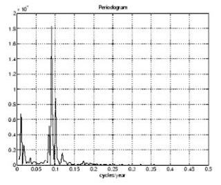
The result of this transform is the complex vector, Y.The magnitude of Y squared is called the power and a plot of power versus frequency is a periodogram. Remove the first component of Y, which is simply the sum of the data, and plot the results:


N = length(Y);
Y(1) = [];
power = abs(Y(1:N/2)).^2;
nyquist = 1/2;
freq = (1:N/2)/(N/2)*nyquist;
plot(freq,power), grid on
xlabel('cycles/year')
title('Periodogram');

The scale in cycles/year is somewhat inconvenient. You can plot in years/cycle and estimate what one cycle is. For convenience, plot the power versus period (where period = 1./freq) from 0 to 40 years/cycle:
period = 1./freq;
plot(period,power), axis([0 40 0 2e7]), grid on
ylabel('Power')
xlabel('Period(Years/Cycle)')

In order to determine the cycle more precisely,


[mp,index] = max(power);
period(index)


ans = 
      11.0769


    As you seen, the result shows that sunspot activity is reaching a maximum about every 11 years. This methods can apply too in many case in meteorology or oceanography that awared happening in cyclic period, for example tide, EL-NINO, etc.